1. Introduction #

Graphs have become increasingly important in machine learning due to their ability to capture complex relationships and dependencies between data points. In particular, graphs have proven to be a powerful tool in processing and understanding event data, which consists of an asynchronous stream of events accompanied by their spatial and temporal information. However, processing and understanding event data poses unique challenges due to its high dimensionality, sparsity, and temporal nature.

One promising approach to processing event data is the Asynchronous Event Graph Neural Network (AEGNN), which effectively utilizes the high temporal resolution provided by event-based cameras to reduce computational time while maintaining accuracy. AEGNN is a novel graph convolutional neural network that leverages the unique properties of event-based cameras to process and understand the rich spatio-temporal information contained in the event data.

In this paper, we reproduce the AEGNN model and evaluate its performance in recognizing objects in the Neuromorphic-Caltech101 dataset. We investigate the impact of changing convolutional operators and hyperparameters on the model’s accuracy. Our results confirm the effectiveness of the AEGNN model in processing event data and highlight the importance of carefully choosing hyperparameters to achieve optimal performance.

Motivation #

Event-based cameras offer high temporal resolution and low power consumption, but pose unique challenges in processing and understanding the rich spatio-temporal information contained in the event data. Current models for event cameras discard the temporal resolution of events, whereas the Asynchronous Event Graph Neural Network (AEGNN) proposed in this paper effectively utilizes the high temporal resolution provided by event-based cameras to largely reduce computational time while maintaining accuracy. The AEGNN model is a novel approach to leverage the unique properties of event-based cameras.

2. Setup #

In the following section, the training and testing platform of AEGNN are described in detail. Given the limited number of computational resources available, some simplifications are made to the training pipeline.

Code & Environment setup #

In order to host the project, Google Compute cloud services are used. Based on the paper’s recommendations, we create an image of a deep learning virtual machine together with a NVIDIA T4 / P100 GPU, which has 16GB RAM. Moreover, the machine was configured with 2 vCPUs and 8gb RAM. This allows us to use VSCode’s ssh feature to remotely connect to the virtual machine from our local computers. The following tutorial is used to set up our editor environment. Code changes and running experiments are performed in this flexible way, by completely isolating the Google Cloud setup, treating it as an external computing machine.

The original author’s code is available on github. However, upon first inspection, the training pipeline is missing. The training script can be found in a separate fork of the original repository (link). This script is then used as a baseline to train the model for the remainder of the project. Our project and code is hosted on GitHub as well (link).

Assumptions & Challenges #

As mentioned, a simplification is necessary during the preprocessing phase, that is subsampling is reduced from 10k to 1k points per sample. Because of GPU cost limitations, the subsampling factor has been reduced for two reasons. First, to speed up training, and secondly, enabling training with a batch size of 16 (as indicated by the paper), and removing the need of a 24GB VRAM GPU.

When running the existing code in the proposed cloud VM, a couple of challenges need to be addressed. With the supplied conda environment file in the existing repository, there is uncertainty about which exact packages the author used for training the model, as well as compatibility problems.

Therefore, the pytorch geometric (PyG) installed behaves differently compared to the code written by the author. The first bug encountered had to do with the subsampling of both spatio-temporal position vector and polarity vector of the events. In the following class method of NCaltech101 class (link to code line), on line 11, after the first iteration of the for loop, the if statement inside the for loop will be False, when trying to subsample the spatio-temporal vectors. This is because the on the first iteration, the polarity vector is subsampled successfully, and therefore data.num_nodes attribute is changed. Saving the original data.num_nodes a scope higher into a variable original_num_nodes and changing the if statement on line 12, solves the problem.

 1
 2
 3
 4
 5
 6
 7
 8
 9
10
11
12
13
14
15
16
17
18
19
20
21

def pre_transform(self, data: Data) -> Data:
        params = self.hparams.preprocessing
        # FIX, save data.num_nodes original here
        # original_num_nodes = data.num_nodes
        
        # Cut-off window of highest increase of events.
        window_us = 50 * 1000
        t = data.pos[data.num_nodes // 2, 2]
        index1 = torch.clamp(torch.searchsorted(data.pos[:, 2].contiguous(), t) - 1, 0, data.num_nodes - 1)
        index0 = torch.clamp(torch.searchsorted(data.pos[:, 2].contiguous(), t-window_us) - 1, 0, data.num_nodes - 1)
        for key, item in data:
            if torch.is_tensor(item) and item.size(0) == data.num_nodes and item.size(0) != 1:
                data[key] = item[index0:index1, :]
                # Coarsen graph by uniformly sampling n points from the event point cloud.
        data = self.sub_sampling(data, n_samples=params["n_samples"], sub_sample=params["sampling"])

        # Re-weight temporal vs. spatial dimensions to account for different resolutions.
        data.pos[:, 2] = normalize_time(data.pos[:, 2])
        # Radius graph generation.
        data.edge_index = radius_graph(data.pos, r=params["r"], max_num_neighbors=params["d_max"])
        return data

Weights and Biases is a popular monitoring tool for training machine learning models. This is used as well by the original authors to observe and log performance during training. After attaching wandb as logger in the pytorch lightning trainer, we save the model at every checkpoint after validation. This enables us to retrieve the last best performing model for to use for inference.

In the following code block, the whole model is serialised as a pickle object together with the learned weights and biases and saved to a pickle file. The issue here, is that the wandb logger is not serialisable in the package version created by us. Thefore, one simple fix is the one presented in the comments. We deepcopy the model without the logger and save it.

 1
 2
 3
 4
 5
 6
 7
 8
 9
10
11
12
13
14

class FullModelCheckpoint(pl.callbacks.ModelCheckpoint):
    FILE_EXTENSION = ".pt"

    def _save_model(self, trainer: pl.Trainer, filepath: str) -> None:
        trainer.dev_debugger.track_checkpointing_history(filepath)
        if trainer.should_rank_save_checkpoint:
            self._fs.makedirs(os.path.dirname(filepath), exist_ok=True)
            
        # trainer_to_save = copy.deepcopy(trainer)
        # trainer_to_save.logger = False
        
        # change to torch.save(trainer_to_save.model, filepath)    
        torch.save(trainer.model, filepath)
        logging.debug(f"Save model checkpoint @ {filepath}")

3. Implementation #

Dataset interpretation #

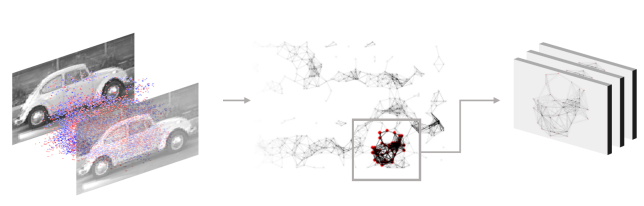
The paper uses three neuromorphic datasets for their experiments: Neuromorphic-Caltech101, Neuromorphic-Cars, and Gen1. The general representation of these datasets is through an event stream, where each event is represented by its pixel coordinates, timestamp (microseconds), and polarity (-1 or 1): \(e_i = (x_i, y_i, t_i, p_i)\)

N-Cars and Gen1 datasets are real-life datasets and thus more complex than N-Caltech101. As such, they are out of scope for our reproduction. However, N-Caltech101 dataset is an event-based adaption of the image-based Caltech101 dataset. It containes simpler data: classes for 101 objects for recognition tasks, as well as bounding box annotations for detection. This reproduction focuses on recognition on N-Caltech101.

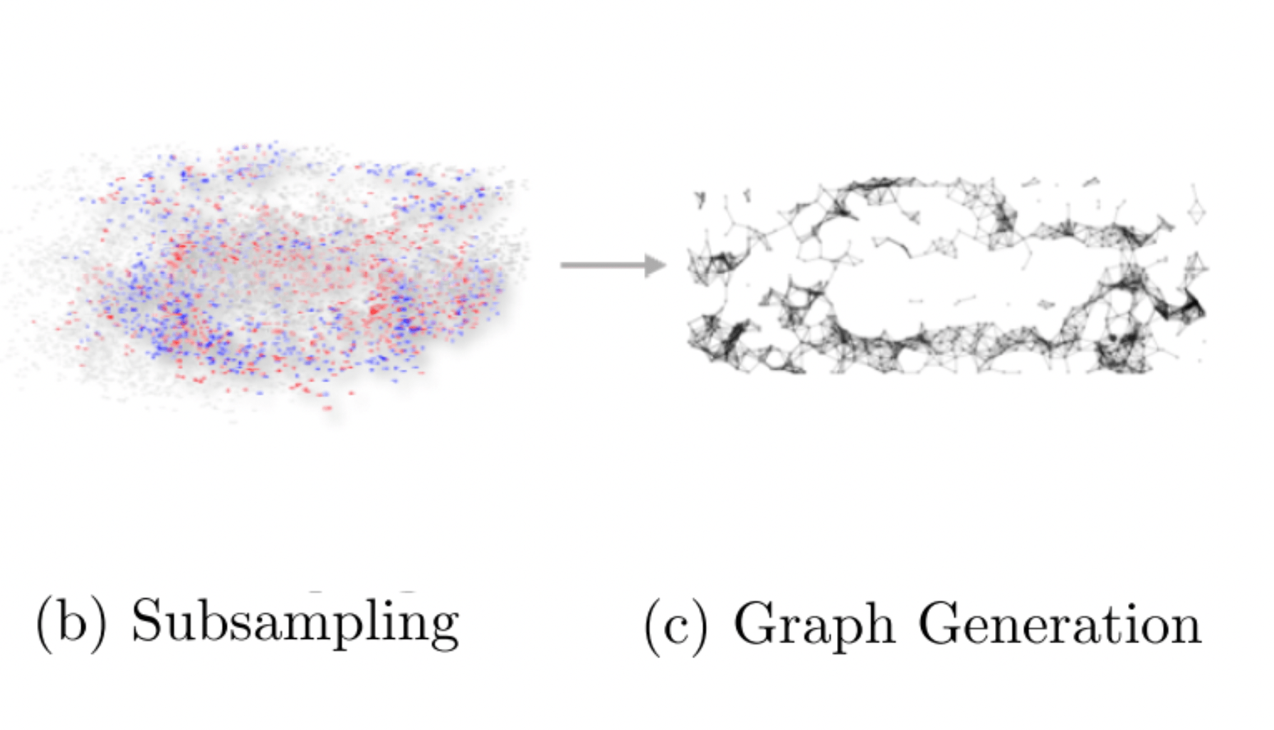
Preprocessing pipeline #

The dataset has to go through some preprocessing steps before training. This improves computation efficiency and results in training and testing phases.

First, events are subsampled to reduce their number and improve efficiency. While the paper uses a sampling of 10000 nodes for their best results, we are using 1000 for better computational efficiency.

Second, these events are used to build an event graph, where each node is an event. Each node is connected to neighbouring nodes within a certain distance \(R\), with a maximum number of neighbours \(D_{max}\). The feature of each node is its event intensity \(p_i\), while each edge is assigned the distance between the nodes it connects, normalized by \(R\).

Training pipeline #

The model is trained on a Google Cloud VM with an NVIDIA T4 / P100 GPU, as explained in Setup Section. We use the Train class from PyTorch Lightning to automate the training procedure and use the following (important) settings:

• Cross Entropy Loss for the multi-class classification task.
• Batch size of 16 as suggested by the paper.
• Adam Optimizer with both learning rate and weight decay of \(5\mathrm{e}{-3}\). The learning rate decreases by a factor of 10 after 20 epochs. Note: our learning rate is 5 times higher than the one suggested by the paper.
• Early stopping when validation loss stops decreasing after 10 epochs.

4. Experiments #

Two main types of experiments are conducted: changing convolutions and hyperparameters evaluation.

Different Convolutions #

The default convolution used by the paper authors is the PyG Spline Convolution. However, since the model is convolution invariant, any type of graph convolution could be applied. We investigate the impact of changing this convolution on the training accuracy.

The model is therefore trained on three types of convolutions: SplineConv (default), GMMConv, and GraphConv. Additionaly, for each convolution type, we train a model with and one without residuals, resulting in a total of 6 models with their corresponding training accuracies.

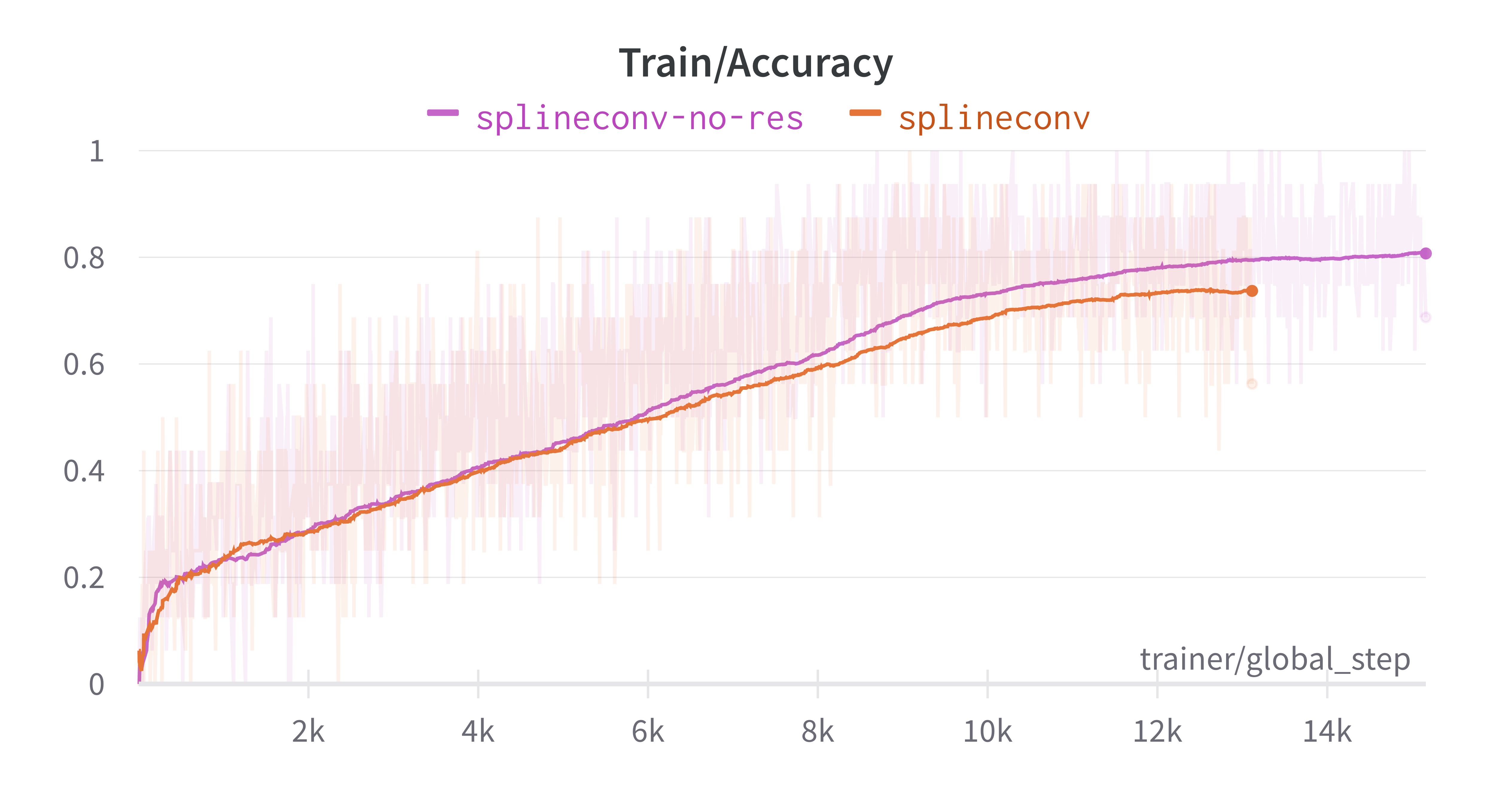
Default Spline Conv #

SplineConv is the spline-based convolutional operator from the SplineCNN paper. It is a generalization of the traditional CNN convolution operator, and aggregates features only in the spatial domain. It has the advantage that it makes the computation time independent from kernel size.

The final values for train accuracy are:

• With residuals: 0.7388
• Without residuals: 0.8073

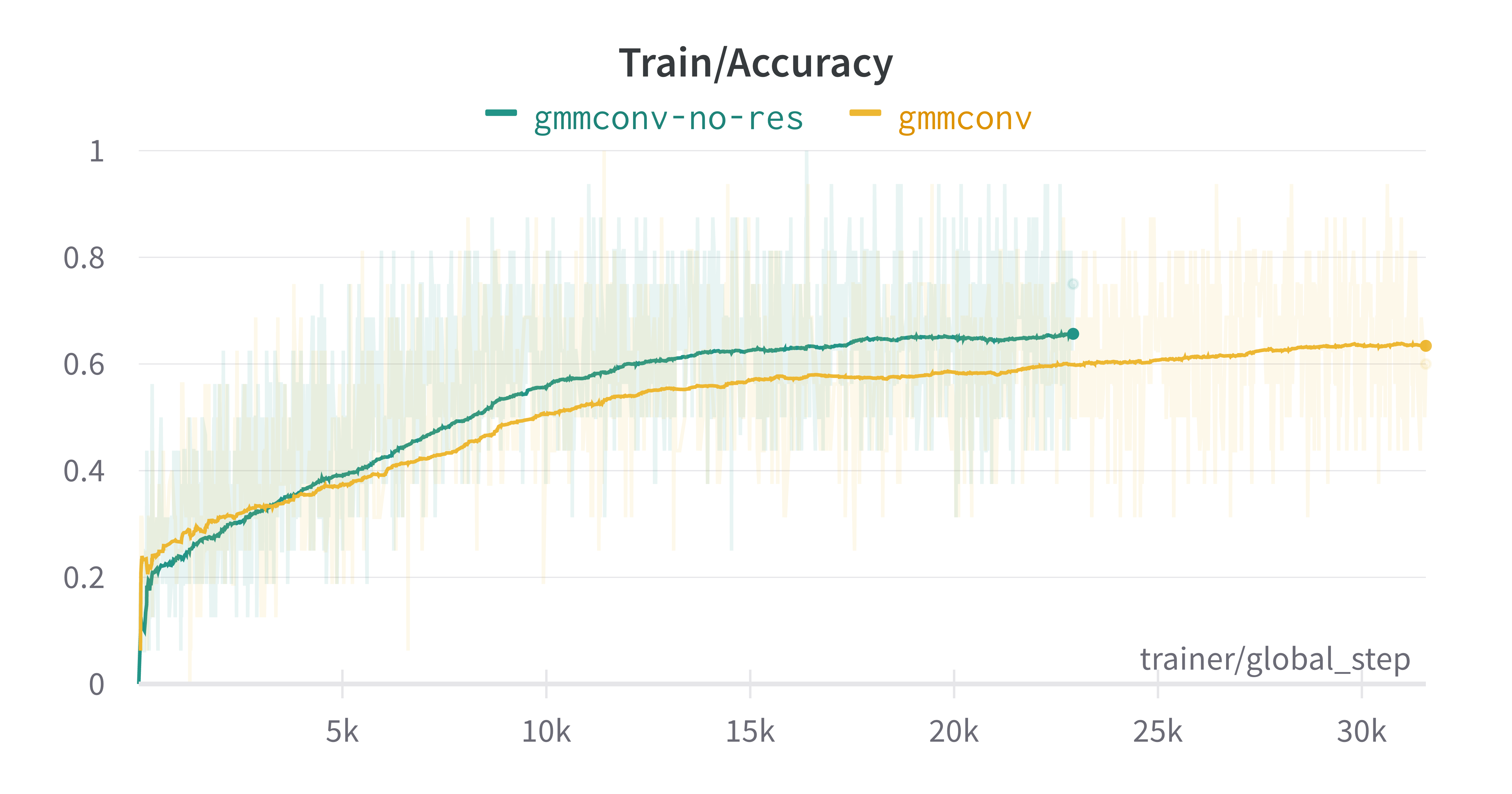
GMMConv #

GMMConv is the gaussian mixture model convolutional operator from the Geometric deep learning on graphs paper. It is applicable on non-Euclidean domains (e.g. manifolds, or graphs in our case), and applies a gaussian assumption to the parametric kernels.

The final values for train accuracy are:

• With residuals: 0.6346
• Without residuals: 0.6709

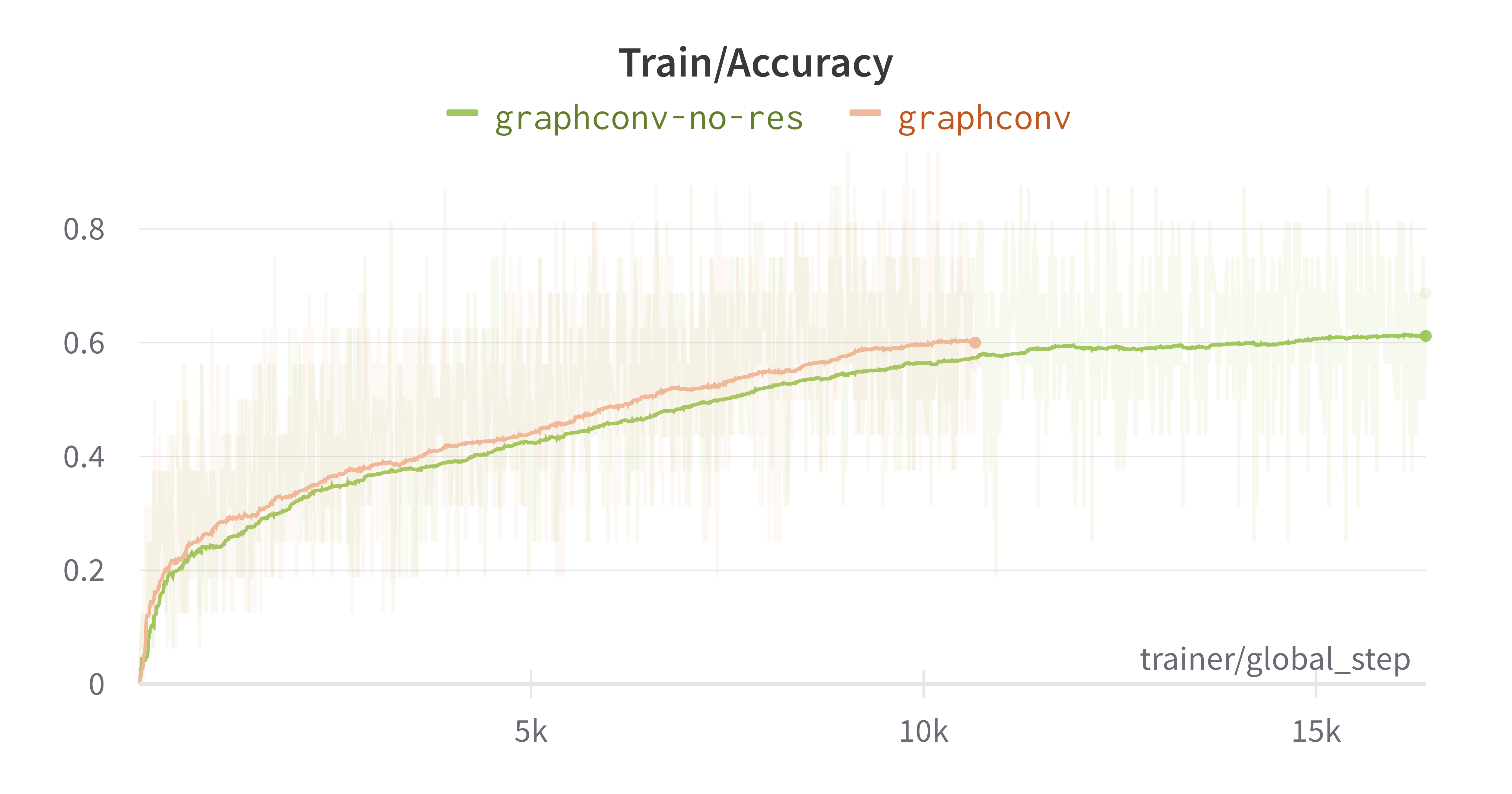
GraphConv #

GraphConv is the graph neural network operator from the Higher-order Graph Neural Networks paper. It performs convolution operations by using the adjacency matrix to compute the weighted sum of node features with their neighbours.

The final values for train accuracy are:

• With residuals: 0.6001
• Without residuals: 0.6117

Analysis #

The final results from the above figures show that, for each convolution type, the models with no residuals performed better than with residuals. The margin between accuracies with and without residuals is relatively small, but consistently in favor of no residuals – around 0.07, 0.02 and 0.01. This indicates the model is too shallow and the data is simple enough (remember our subsampling value is 10 times smaller than the paper’s) to generalize without residual connections. If the model were deeper, more degradation would occur, which would be fixed with residuals.

Additionally, this experiment confirms the paper’s choice of SplineConv operator over other operators. The accuracies obtained for SplineConv in both cases (residuals and no residuals) are much higher than the other two convolutions.

Hyperparameter evaluation #

Basics #

In this section, we will conduct a analysis to investigate the impact of hyperparameters on the model’s performance, specifically focusing on detection accuracy. Our primary interest lies in understanding how varying hyperparameters can influence the model’s capabilities. However, due to constraints in computational resources, we will limit our testing to the ’ncaltech101’ dataset instead of extending it to the full range of datasets, which includes NCars, NCaltech101, and Prophesee Gen1 Automotive.

For the purpose of this analysis, we have chosen to concentrate on a single hyperparameter, the spatio-temporal distance \(R\). This decision allows for a more in-depth examination of the chosen hyperparameter and its effects on the model. In the context of the model, for each pair of nodes \(i\) and \(j\), an edge \(e_{ij}\) is generated between them only if the spatio-temporal distance between the nodes meets the following criterion: \(R \geq ||X_i -X_j||\)

Experiment description #

In the research paper, the spatio-temporal distance parameter \(R\) serves a crucial purpose in regulating the number of connected nodes within the model, thus striking a balance between computational cost and accuracy. This balancing act is essential to ensure that the model operates efficiently without compromising the quality of its performance.

In our experiment, however, our primary focus is to dive deeper into the relationship between \(R\) and the model’s accuracy. As a result, we will not be considering the impact of \(R\) on computational resources in this particular analysis.Table below, shows the value space we used to test the model. The table below shows the value space we used to test the model. It is worthed mentioning that \(R=5, D_{max} =32， batchsize= 16\) is the parameter used in the paper. Due to the computational cost limitation, the \(n_{samples}\) is decreased to \(2,500\) instead of \(25,000\) in the paper.

Table 1: The tested value space of \(R\), \(D_{max}\) is maximal number of neighborhood nodes,i.e \(|\mathcal{N}(i)\leq D_{max}|\), \(n_{samples}\) is the number of samples.

Result and analysis #

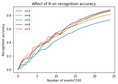
The figure above presents the experimental results of recognition accuracy for different values of the spatio-temporal distance parameter, \(R\). It is evident from the results that, in all cases, the model does not attain its optimal performance due to the limitations imposed by the number of events. Interestingly, we also observe a trend where a decrease in the \(R\) value corresponds with a decrease in recognition accuracy. This correlation becomes more pronounced as the number of events increases.

From these observations, we can draw the conclusion that the spatio-temporal distance \(R\) has a significant impact on the model’s performance. Generally, larger \(R\) values tend to yield better performance. However, it is essential to consider the trade-off between accuracy and computational cost. As the \(R\) value increases, so does the potential for higher computational costs, which can be a limiting factor when optimizing the model.

5. Conclusion #

The Asynchronous Graph Neural Network Model (AEGNN) model is reproduced in a Google Cloud environment, using existing source code and some minor changes. The preprocessing and training pipelines are adapted to perform two types of experiments: changing convolutions and hyperparameters evaluation.

The first experiment tests three types of convolutions and use of residual connections, and concludes the residuals are not needed when sampling low number of events. Additionaly, it confirms that the paper’s choice of spline convolutions is the best performing.

The second experiment shows the impact of varying spatio-temporal distance \(R\) values on training recognition accuracy. The larger \(R\) value tends to have higher accuracy in recongition however it may also leads to higher computational cost.

These results are achieved under some computational tradeoffs that definitely influence accuracies obtained. For future work, the impact of higher events sampling with different convolutional operators is worth exploring.